


Data Cleaning SQL- BigQuery
Project 1
Information: This is a customer data set with customer names, IDs, addresses, cities, states, zip codes, and countries. This Data set was given to me through the Google Data Analytics Professional Certification Course.
Steps Taken:
1. Downloaded dataset into SQL BigQuery
2. I was asked to add a customer to the dataset and I added a row of data using the INSERT INTO and VALUES functions in this query:
INSERT INTO
`my-first-project-sql-363013.customer_data.customer_adress`
(customer_id, address, city, state, zipcode, country)
VALUES
(2645,'3456 Highfield Court', 'Jackson', 'MI',49202, "US")
3. I was asked to update a current customer address so I updated it using this query
UPDATE
`my-first-project-sql-363013.customer_data.customer_adress`
SET
address = '2346 New Haven Ct'
WHERE
customer_id = 4957
4. I wrote this next query to find out if there were any mistakes in the data and found some rows were showing a LENGTH of 3 and not 2 in the country row
SELECT
LENGTH(country) AS letters_in_country
FROM
`my-first-project-sql-363013.customer_data.customer_adress`
5. I wrote this query to find the mistake where LENGTH was 3 and not 2
SELECT
country
FROM
`my-first-project-sql-363013.customer_data.customer_adress`
WHERE
LENGTH(country) > 2
6. I found that someone imputed ‘USA’ Instead of ‘US’ in this query
SELECT
country
FROM
`my-first-project-sql-363013.customer_data.customer_adress`
WHERE
LENGTH(country) > 2
7. In order to view the customer_id with ‘US’ and ‘USA’ in the country column I used the SUBSTRING function and the DISTINCT function because there are duplicate customer_id in this query:
SELECT
DISTINCT customer_id
FROM
`customer_data.customer_adress`
WHERE
SUBSTRING(country, 1, 2) = "US"
8. I then write this query to find out if the same mistake has been made in the state column
SELECT
state
FROM
`my-first-project-sql-363013.customer_data.customer_adress`
WHERE
LENGTH(state) > 2
9. I find out that one OH has extra whitespace behind it and I use the trim function in the query to trim the whitespace
SELECT
DISTINCT customer_id
FROM
`customer_data.customer_adress`
WHERE
TRIM(state)='OH'
Information: This is a data set with information on the number of doors, fuel type, horsepower, etc.
Description of data: https://archive.ics.uci.edu/ml/datasets/Automobile
1. Download data onto BigQuery
2. Inspected data to make sure it matched the description using this query
SELECT
DISTINCT fuel_type
FROM
Cars.car_info
3. I found it matched the description so I moved on to see if the min and max length are the same as the description using this query
SELECT
MIN(length) AS min_length,
MAX(length) AS max_length
FROM
Cars.car_info
4. I then look for ‘null’ values in the num_of_doors
SELECT
*
FROM
Cars.car_info
WHERE
num_of_doors IS NULL
5. I find that there are 2 null values and checked with stakeholders and found that all the null values should be say “four” so I write this query to fill in the null
UPDATE
Cars.car_info
SET
num_of_doors = "four"
WHERE
make = "dodge"
AND fuel_type = "gas"
AND body_style = "sedan"
6. I do further inspection and use this query
SELECT
DISTINCT num_of_cylinders
FROM
Cars.car_info
7. I find out that instead of ‘two’ one of the cells says ‘tow’ so I write this query to change it
UPDATE
Cars.car_info
SET
num_of_cylinders = "two"
WHERE
num_of_cylinders = "tow"
8. I now inspect the compression ratio column the see if the range is between 7 and 23 like the data description says so I run this query
SELECT
MIN(compression_ratio) AS min_compression_ratio,
MAX(compression_ratio) AS max_compression_ratio
FROM
Cars.car_info
9. I find out that the max is 70 and this should be deleted (after I consult the stakeholder and manager) so I write this query to remove it.
DELETE
Cars.car_info
WHERE
compression_ratio = 70
10. I then check the drive_wheels column to check for consistency using this query:
SELECT
DISTINCT drive_wheels
FROM
Cars.car_info
11. I find that 4wd shows up twice as a distinct input so I write this query to find out why
SELECT
DISTINCT drive_wheels,
LENGTH(drive_wheels) AS string_length
FROM
Cars.car_info
12. I find out that multiple of the 4wd has 4 lengths so I write this query to fix that
UPDATE
Cars.car_info
SET
drive_wheels = TRIM(drive_wheels)
WHERE TRUE
Data Cleaning in SQL- BigQuery
Project 2
Data Analysis SQL- BigQuery
Project 1 - Getting to know the data with sorting and filtering
Information: This is data from the Google Data Analytics coursework. It is a list of movies, release dates, revenue, etc.
1. Filter the data to only show the comedy Genre that made more than $500,000,000
SELECT
Movie_Title, Genre, Revenue `movie_data.movies`
FROM
`movie_data.movies`
WHERE
Genre = 'Comedy'
AND
Revenue>500000000
2. Sort the data by release date ( DECS) and filter the to only show the comedy genre.
SELECT
*
FROM
`movie_data.movies`
WHERE
Genre = 'Comedy'
ORDER BY
Release_Date
DESC
3. What was the average revenue in the comedy genre?
SELECT
AVG(Revenue) AS average_comedy_rev
FROM
`my-first-project-sql-363013.movie_data.movies`
WHERE
Genre = "Comedy"
4. What genre had the highest average revenue?
SELECT
Genre,
AVG(Revenue) AS average_rev
FROM
`my-first-project-sql-363013.movie_data.movies`
GROUP BY
Genre
ORDER BY
average_rev
DESC
Here is the result:

Project 2 - Using JOINs and subqueries
Information: This data is from a bike share app, from BigQuery, I will show the questions the Stakeholders asked and then what query I wrote to find the answer.
1. Compare the average number of bikes available at each station to the average number of bikes available at individual stations.
SELECT
station_id,
num_bikes_available,
(
SELECT
AVG(num_bikes_available)
FROM
`bigquery-public-data.new_york.citibike_stations`
)
AS avg_num_bikes_available
FROM
bigquery-public-data.new_york.citibike_stations
This is the result:
2. Find the start stations with the most number of rides.
SELECT
station_id,
name,
num_of_rides AS number_of_rides_at_station
FROM
(
SELECT
start_station_id,
COUNT(*) num_of_rides
FROM
`bigquery-public-data.new_york.citibike_trips`
GROUP BY
start_station_id
)
AS station_num_trips
INNER JOIN
`bigquery-public-data.new_york.citibike_stations` ON station_id = start_station_id
ORDER BY
station_num_trips.num_of_rides DESC
This is the result:
3. What were the 10 most popular trips (start location to end location) and what was the average time of those trips?
SELECT
CONCAT (start_station_name,"to", end_station_name) AS route,
COUNT (*) AS num_trips,
ROUND (AVG (CAST (tripduration AS int64) / 60) ,2) AS duration
FROM
`bigquery-public-data.new_york.citibike_trips`
GROUP BY
start_station_name,end_station_name
ORDER BY
num_trips DESC
LIMIT
10
This is the result:


Tableau Visualizations
Project 1 - Electric Cars in Washington State
Information: This data is from data.gov and it shows the Battery Electric Vehicles (BEVs) and Plugin Hybrid Electric Vehicles (PHEVs) that are currently registered through the Washington State Department of Licensing (DOL).
Key insights:
1. The Jaguar has the highest Electric Range out of any of the other electric cars with a top range of 212.1 miles
2. The clear winning of the most popular electric car in Washington State is Tesla (47,264), followed by Nissan (12,909), and then Chevrolet (9,846).
3. The highest population of electric cars in Washington State is in Seattle.
4. The most popular Tesla in Washinton State is the Model 3.
Click on the picture to open up Tableau and interact with the Visualization
Project 2 - World Happiness
Information: This data is from the Google Data Analytics coursework. The data looks at elements of happiness and quantifies them. I took the data and made visualizations that compared the elements to find out what really made people happy as well as looked at European happiness as well.
Key Insights:
1. The top 4 things that influence a country's happiness are; GDP, family, freedom, and life-expectancy
2. Europe, overall, was a happier nation and had higher correlations between family and happiness, life expectancy and happiness, and GDP and happiness than compared to the rest of the world.
3. The happiest country according to the data was a 4-way tie with; Norway (7.5), Denmark (7.5), Iceland (7.5), and Switzerland (7.5).
Click on the picture to open up Tableau and interact with the Visualization.
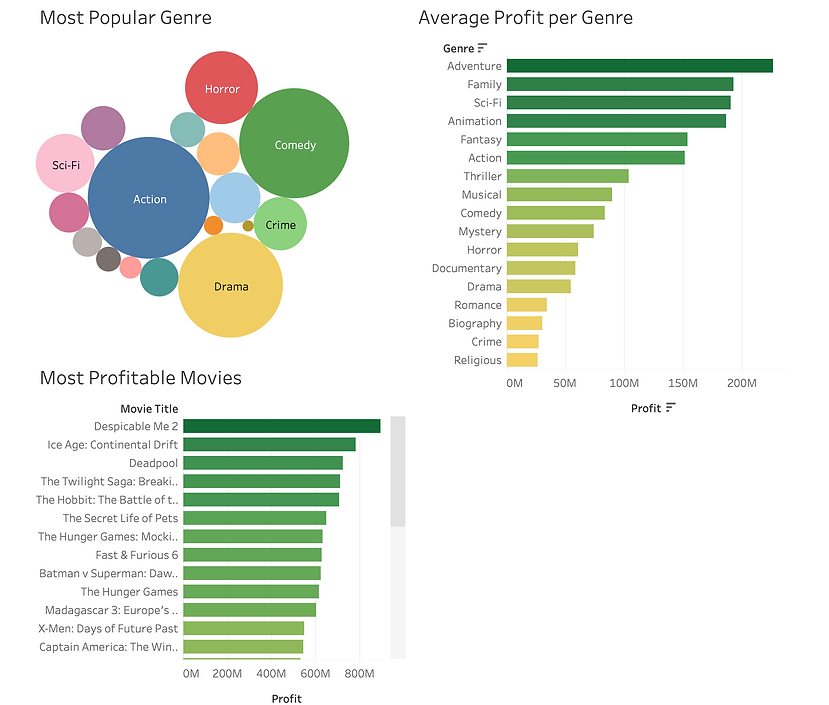
Project 3- Movies
Information: This data is from the Google Data Analytics coursework. The data includes revenue, budget, movie titles, etc.
Key Insights:
1. The 3 most popular Genres of movies made were #1 Action, #2 Comedy, and #3 Drama.
2. The most profitable Genres were #1 Adventure, #2 Family, and #3 SciFi. Where Action, Comedy, and Drama come in at #6 (Action), #9 (Comedy), and #12 (Drama).
3. The most profitable move was Despicable Me 2 at $894,800,000


R Visualizations
Project 1 - Palmer Penguins
Information: This data is from posit cloud and is called "palmerpenguins".
Key insights:
-
Male penguins are larger on average
-
Gentoos are the largest penguins
-
As flipper length goes up, so does body mass
-
Adelie penguins are more spread out in size than the chinstrap penguins
Visual 1 code:
ggplot(data = penguins) +
geom_point(mapping = aes(x=flipper_length_mm, y = body_mass_g,color=species))+
facet_grid(~sex)
Visual 2 code:
ggplot(data = penguins) +
geom_point(mapping = aes(x=flipper_length_mm, y = body_mass_g,color=species))+
facet_wrap(~species)
Visual 3 code:
ggplot(data = penguins) +
geom_smooth(mapping = aes(x=flipper_length_mm, y = body_mass_g)) +
geom_point(mapping = aes(x=flipper_length_mm, y = body_mass_g,color = species))
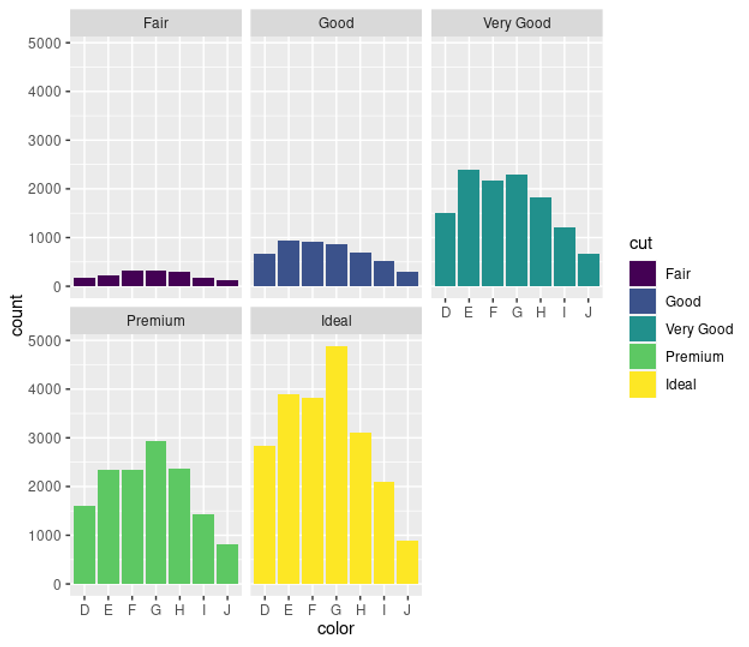
Project 2 - Diamonds
Information: This data is from posit cloud and is called "diamonds".
Visual 1 Code:
ggplot(data = diamonds)+
geom_bar(mapping=aes(x=cut,fill=clarity))
Visual 2 code:
ggplot(data = diamonds)+
geom_bar(mapping=aes(x=color,fill=cut))+
facet_wrap(~cut)


R Cleaning and Analysis
Project 1 - Palmer Penguins
Information: This data is from posit cloud and is called "palmerpenguins".
1. Rename the island column new_island
Code Chunk:
penguins %>%
rename(island_new=island)
2. Change all the column names to uppercase
Code Chunk:
rename_with(penguins,toupper)
3. Add a row at the end to calculate kgs for body mass and meters for body length
Code Chunk:
penguins %>%
mutate(body_mass_kg=body_mass_g/1000, flipper_length_m=flipper_length_mm/1000)
4. Arrange the data by bill length smallest to largest
Code Chunk:
penguins %>% arrange(-bill_length_mm)
5. Show the average bill length for each island
Code Chunk:
penguins %>% group_by(island) %>% drop_na() %>% summarize (mean_bill_length_mm = mean (bill_length_mm))
Result:
island mean_bill_length_mm
<fct> <dbl>
1 Biscoe 45.2
2 Dream 44.2
3 Torgersen 39.0
6. Show max and min bill length for each island
Code Chunk for max:
penguins %>% group_by(island) %>% drop_na() %>% summarise(max_bill_length_mm = max(bill_length_mm))
Result:
island max_bill_length_mm
<fct> <dbl>
1 Biscoe 59.6
2 Dream 58
3 Torgersen 46
Code Chunk for min:
penguins %>% group_by(island) %>% drop_na() %>% summarise(min_bill_length_mm = min(bill_length_mm))
Result
island min_bill_length_mm
<fct> <dbl>
1 Biscoe 34.5
2 Dream 32.1
3 Torgersen 33.5
7. Show to average bill length for each species on each island
Code Chunk:
penguins %>% group_by(species, island) %>% drop_na() %>% summarise(max_bl=max(bill_length_mm), mean_bl = mean(bill_length_mm))
Result:
species island max_bl mean_bl
<fct> <fct> <dbl> <dbl>
1 Adelie Biscoe 45.6 39.0
2 Adelie Dream 44.1 38.5
3 Adelie Torgersen 46 39.0
4 Chinstrap Dream 58 48.8
5 Gentoo Biscoe 59.6 47.6